
6.2. Applied Stochastic Analysis’s home work 2
6.2.1. No.1
omitting..
6.2.2. No.2
Testify the half order convergence of MC through a numerical example.
Here is the code:
 1function ans=hw2_2()
 2for i = 1:10
 3    res(i)=estimate();
 4end
 5ans = mean(res);
 6
 7end
 8
 9function ans=estimate()
10syms x;
11f = sin(pi*x);
12I = int(f,0,1);
13N = [4,8,16,32,64,128,256,512]*10;
14for i = 1:8
15    res(i)=I-mc(N(i),f,x);
16end
17res=abs(double(res));
18ans=polyfit(log(N),log(res),1);
19ans = -ans(1);
20end
21
22function ans=mc(n,f,x)
23
24ans = mean(subs(f,x,rand(n,1)));
25end
6.2.3. No.3
How many ways can you give to construct the uniform distribution on \(S^2\) . Implement them and make a comparison.
Set \(\theta\) and \(\phi\) be the spherical coordinates. Here I got three mechod:
Let \(\theta\) be the uniform distribution of \([0,2\pi)\) and \(P_{\phi}=\frac{1}{2}sin\phi\)
pick \(u=cos\phi\) to be uniformly distributed on \([-1,1]\), and \(\theta\) the same as above.
Marsaglia (1972) derived an elegant method that consists of picking \(x_1\) and \(x_2\) from independent uniform distributions on \((-1,1)\) and rejecting points for which \(x_1^2+x_2^2\geq 1\) . From the remaining points.
Here is the code:
 1function hw2_3()
 2
 3    num =10000;
 4    subplot(2,2,1);
 5    [a,b,c]=sphere();
 6    mesh(a,b,c);
 7    hold
 8    Title('Method a');
 9    tic
10    [x,y,z]=sphere1(num);
11    toc
12    plot3(x,y,z,'.');
13
14
15    subplot(2,2,2);
16    [a,b,c]=sphere();
17    mesh(a,b,c);
18    hold
19    Title('Method b');
20    tic
21    [x,y,z]=sphere2(num);
22    toc
23    plot3(x,y,z,'.');
24
25    subplot(2,2,3);
26    [a,b,c]=sphere();
27    mesh(a,b,c);
28    hold
29    Title('Method c');
30    tic
31    [x,y,z]=sphere3(num);
32    toc
33    plot3(x,y,z,'.');
34end
35
36function [x,y,z]=sphere1(n)
37    x=zeros(1,n);
38    y=zeros(1,n);
39    z=zeros(1,n);
40    for i=1:n
41        theta = 2*pi*rand;
42        phi = acos(1-2*rand);
43        s = sin(phi);
44        x(i) = cos(theta)*s;
45        y(i) = sin(theta)*s;
46        z(i) = cos(phi);
47    end
48end
49
50function [x,y,z]=sphere2(n)
51
52    x=zeros(1,n);
53    y=zeros(1,n);
54    z=zeros(1,n);
55    for i=1:n
56
57        theta = 2*pi*rand;
58        u = rand*2-1;
59        s = sqrt(1-u^2);
60        x(i) = s*cos(theta);
61        y(i) = s*sin(theta);
62        z(i) = u;
63    end
64
65end
66
67function [x,y,z]=sphere3(n)
68
69    x=zeros(1,n);
70    y=zeros(1,n);
71    z=zeros(1,n);
72    for i=1:n
73
74        x1 =2*rand-1;
75        x2 =2*rand-1;
76        p = x1^2+x2^2;
77        while p>=1
78            x1 =2*rand-1;
79            x2 =2*rand-1;
80            p = x1^2+x2^2;
81        end
82        s =sqrt(1-p);
83        x(i) = 2*x1*s;
84        y(i) = 2*x2*s;
85        z(i) = 1-2*p;
86    end
87end
And here is the result:
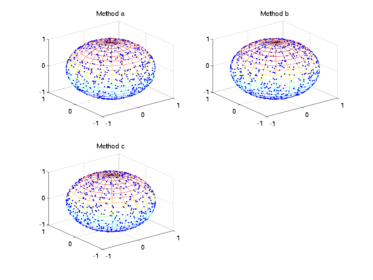
It’s obvius that the method c is the most effient, but not stable.
a: Elapsed time is 0.026833 seconds.
b: Elapsed time is 0.020886 seconds.
c: Elapsed time is 0.006588 seconds.
PS: I. Another easy way to pick a random point on a sphere is to generate three Gaussian random variables. #. Cook (1957) extended a method of von Neumann (1951) to give a simple method of picking points uniformly distributed on the surface of a unit sphere. This method only need multiply add, sub and divide.